Getting started#
Table of Contents
Installation#
pyH2A can be installed using pip:
pip install pyH2A
Choose configuration#
First, the configuration of the hydrogen production technology should be specified. This is done by selecting the appropiate plugins, which together form the desired production pathway. For example, in case of photovoltaic + electrolysis (PV+E), the Hourly_Irradiation_Plugin and Photovoltaic_Plugin may be used: Hourly_Irradiation_Plugin models the irradiation in specified location, while Photovoltaic_Plugin models electricity production using PV based on the hourly irradiation data and subsequent production of hydrogen from electrolysis. Changing the plugins changes the technology configuration and new configurations (e.g. including battery storage) can be modelled by creating new plugins (see Plugin Guide for information on how to create new plugins).
The chosen plugins are specified in the Workflow table of the input file:
# Workflow

Name | Type | Position
--- | --- | ---
Hourly_Irradiation_Plugin | plugin | 0
Photovoltaic_Plugin | plugin | 0
Name is the name of the used module, Type is the type of module (in both cases plugin) and Posiition refers to the the position in the workflow when this module is executed (in this case both positions are 0, meaning that these plugins are executed at the beginning of the workflow with Hourly_Irradiation_Plugin being executed before Photovoltaic plugin). See Default Settings for the default positions of the different elements of the workflow.
At this point one may also specify the analysis modules which are to be used. These are included by putting a header with the name of the analysis module into the input file.
# Monte_Carlo_Analysis
This header request the Monte_Carlo_Analysis module.
Generate input file template#
The input file containing the Workflow tabe and possible analysis headings is the starting point to generate the full input file template.
At this point the input file may look like this:
# Workflow

Name | Type | Position
--- | --- | ---
Hourly_Irradiation_Plugin | plugin | 0
Photovoltaic_Plugin | plugin | 0

# Monte_Carlo_Analysis
In the current directory, the generate function from the pyH2A command line interface may be used to generate the full input file template:
pyH2A generate -i input.md -o input_full.md --origin --comments
The --origin flag includes information in the template on which plugin/module has requested a given input. The --comments flag includes additional information on the requested input (from the documentation). The flags can be omitted to obtain a cleaner input file template.
The thus generated file input_full.md can be used to enter the model information.
Enter model information#
The input file template specifies which model information has to be entered for the selected technology configuration. For example, Hourly_Irradiation_Plugin requests a file containg hourly irradiation data:
# Hourly Irradiation

Parameter | Value | Comment Value
--- | --- | ---
File | str | Path to a `.csv` file containing hourly irradiance data as provided by https://re.jrc.ec.europa.eu/pvg_tools/en/#TMY, ``process_table()`` is used.
str indicates that a string which a path to the file is requested (regular Python types are used for input prompts, such as str, int, float, ndarray etc.).
Other tables allow for flexible processing of input information, which is indicated by the placeholder [...]. For example, the default Capital_Cost_Plugin creates this input prompt:
# [...] Direct Capital Cost [...]

Parameter | Value | Comment Value
--- | --- | ---
[...] | float | ``sum_all_tables()`` is used.
The leading and ending [...] indicates a table group, meaning that all tables containing the center string in their heading will be processed together (in case of Direct Capital Cost this can for example be used to break up the information on direct capital costs into seperate tables for easier readability and subsequent cost breakdown analysis).
The [...] in the Parameter column indidcates that any parameter name can be chosen here and any number of parameters can be entered into the table. sum_all_tables() means that all the information will ultimately be summed up to compute the total capital cost.
Instead of entering actual values, it is also possible to enter references to other parts of the input file, using the table > row > column synthax. This kind of reference can either be entered directly into the prompted input field (for example entering it in the Value column of Direct Capital Cost table), or Path column can be added. For example:
# Electrolyzer

Name | Value
--- | ---
Nominal Power (kW) | 5,500.0
...

# Photovoltaic

Name | Value | Path
--- | --- | ---
Nominal Power (kW) | 1.5 | Electrolyzer > Nominal Power (kW) > Value
...
In this case, the Path column of Photovoltaic > Nominal Power (kW) > Value references Electrolyzer > Nominal Power (kW) > Value. Because the reference is in the Path column, the referenced value is multiplied by the value in Photovoltaic > Nominal Power (kW) > Value. In this case, use of referencing ensures that the photovoltaic nominal power is a factor of 1.5 higher than the electrolyzer nominal power (and it is automatically updated when the electrolyzer nominal power is changed).
Run pyH2A#
Once all the model information has been entered, pyH2A can be run to perform the actual techno-economic analysis. This can be done using the command line interface:
pyH2A run -i input_full.md -o .
-i specifies the path of the input file (in this example the input file is in the current directory) and -o specifies the output directory (. means the current directory is selected for the output).
Upon completion, pyH2A prints the levelized cost of hydrogen, for example:
Levelized cost of hydrogen (base case): 3.5777931317137512 $/kg
Generate plots, save results, access information#
The power of pyH2A lies in the ability to interface the core techno-economic analysis with different analysis modules to perform in-depth analysis of the results. For example, when the Monte_Carlo_Analysis module is requested in the input file, Monte Carlo analysis is performed in which selected input parameters are randomly varied to analyze the future hydrogen cost trajectory. Typically, analysis modules contain methods to generate plots of the analysis results. These are requested by adding a Methods table to the input file. For example:
# Methods - Monte_Carlo_Analysis

Name | Method Name | Arguments
--- | --- | ---
distance_cost_relationship | plot_distance_cost_relationship | Arguments - MC Analysis - distance_cost
Including this table in the input file requests that the plot_distance_cost_relationship() method is executed. Arguments can be passed to the method in the Arguments column. In this case, a simple string is included Arguments - MC Analysis - distance_cost. This directs pyH2A to another table in the input file which contains the method arguments:
# Arguments - MC Analysis - distance_cost

Name | Value
--- | ---
show | True
save | False
legend_loc | upper right
log_scale | False
plot_kwargs | {'dpi': 300, 'left': 0.09, 'right': 0.5, 'bottom': 0.15, 'top': 0.95, 'fig_width': 9, 'fig_height': 3.5}
table_kwargs | {'ypos': 0.5, 'xpos': 1.05, 'height': 0.5}
image_kwargs | {'path': 'pyH2A.Other~PV_E_Clipart.png', 'x': 1.6, 'zoom': 0.095, 'y': 0.2}
This synthax is useful when a number of arguments are provided. Alternatively, a dictionary which arguments can be directly included in the Arguments column:
# Methods - Monte_Carlo_Analysis

Name | Method Name | Arguments
--- | --- | ---
distance_cost_relationship | plot_distance_cost_relationship | {'show': True, 'save': True}
By setting save to True, the plot is saved to the output directory. In this case, the following plot is generated:
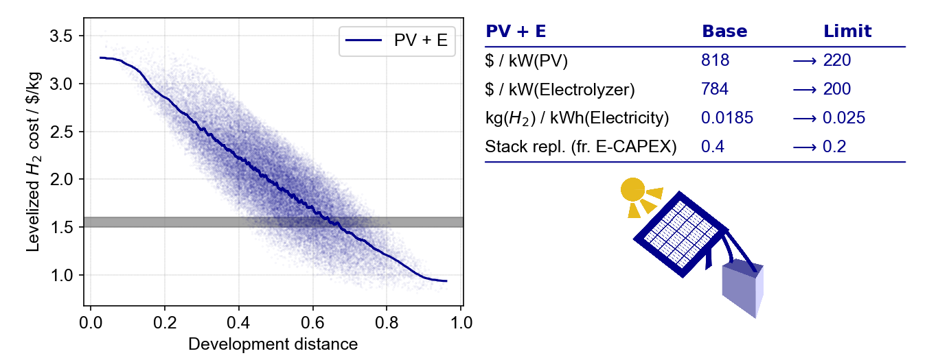
Example output plot from Monte Carlo analysis.#
To access detailed information, which is generated during runtime, pyH2A can also be run from a Python script, which allows for full access to the information. For example:
from pyH2A.run_pyH2A import pyH2A

result = pyH2A('input_full.md', '.')
result is a pyH2A class object. Its attributes contain all the information from the pyH2A run. For example, result.inp is a dictionary with all processed input information, result.base_case contains the information from the discounted cashflow calculation for the specified input information (base case), including all information generated by plugins (accessible via result.base_case.plugs, which is dictionary with all plugin class instances). Furthermore, result.meta_modules is a dictionary which contains all of the analysis module class instances, which were generated during the pyH2A run. With this methodology, pyH2A calculations and results can be integrated into other scripts/programs.